by
by Continuing from my previous post on randomness, I’d like to talk about non-uniform distributions, which certainly don’t get all the love they deserve. When people talk or think about randomness in games, they commonly think about fair distributions. And I know we spent a lot of time in Part 1 actually trying to achieve perfect uniformity because it brings “fairness” to games, but in reality, there are cases where you don’t want your random events to be ruled by a “fair” distribution at all.
Reality Check #4: Sometimes uniformity is bad
Fun fact: For a lot of “random” events in nature, every possible outcome rarely has the same chance of occurring, so perhaps trying to achieve that uniformity in games could be a mistake to begin with.
Let’s take rabbits for instance.
Yes, rabbits.
If you observe the population of rabbits of a given area, you’ll notice that they’ll have a”typical average size”. Let’s call that size X. You’ll find that most rabbits in the area will be around that size. There will be a rare few that are either considerably smaller than X or considerable bigger (outliers), but for the most of it, rabbits will be “just around” X in size. Same goes for any other quantifiable trait that depends on enough factors to be considered random.
They will most-likely follow what is called a Normal (or Gaussian) distribution, which is said to appear in nature all the time. The function that defines this distribution is also called the Gaussian Bell, due to the shape of the curve.
This model has two parameters: an expected value or mean (represented by the Greek letter μ), which is the value that should appear the most in the set, and a standard deviation (σ), which is a measure of how disperse the samples are, relative to the previously defined “average” value.
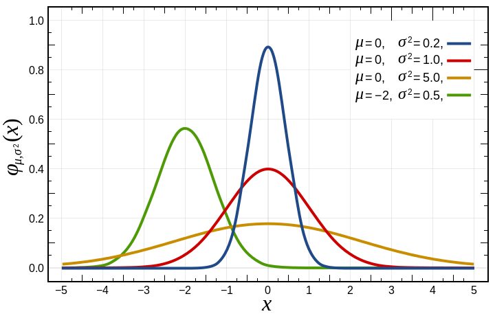
You can see in the graph above several Gaussian distributions with different parameters. A particular case of this curve is known as the standard normal distribution (plotted in red), and is basically a bell curve with an average of 0 and a variance (which is the “standard deviation squared”) of 1.0. These two parameters tell us that we expect values in this distribution to be “around 0” with most of them sitting between -1.0 and 1.0 (one standard deviation away from μ).
In a normal distribution, the interval between μ-σ and u+σ will encompass around 68% of the samples from your set. A smaller value of σ causes this majority to be packed more tightly around the center value, while a bigger deviation has the opposite effect and spreads the possible values over a wider range. In all cases the samples remain centered around the expected “average”.
The more general formula for this model is a bit ugly, especially when expressed in pseudo-C code, so I’ll start with the “standard” normal distribution (where μ and σ have fixed values of 0.0 and 1.0, respectively):
std_norm (x) = exp(-(x*x)/2) / sqrt(2*M_PI)
Where exp(n) is a function that computes “e (Euler’s number) raised to power n”, sqrt(x) is “the square root of x”, and M_PI is, of course, our friend Pi.
As you probably have guessed already (or if you read the article on Wikipedia) you can transform the “standard” normal distribution to any normal distribution of arbitrary μ and σ values very easily. For the sake of simplicity I will call these parameters “m” (mean) and “sd” (standard deviation) instead of their Greek symbols. With that in mind, the formula for this transformation would be as follows:
norm (x, m, sd) = std_norm ((x-mean)/sd) / sd
Please remember that this function represents how frequently we want our different numbers to appear when we draw them from a random generator. We no longer want each number to have an equal chance of being drawn as we previously did with our uniform distribution.
While we won’t need this straight away, it’s worth pointing out that a random variable that follows the normal distribution (called a normal deviate) can also be obtained from another variable that follows the standard normal distribution using the same principle. In this case the transformation is way more straightforward:
norm_deviate (m, sd) = sd*std_norm_deviate() + m
We are still a few steps away from generating random numbers in a way that follows a Gaussian curve, but before things get more confusing let’s bring the new concepts we learnt back to our example:
If you are trying to create a random population of creatures in your game, and you are using LCG or any PRNG where every number has equal probabilities of being chosen on the long run, your results will be weird, to say the least. The “rare” sizes will not really be rare as they’ll have equal chances or being chosen and disastrously wild chances of appearing in small groups. Even if you hard-code certain “probability” of a group or size to occur in your game, comparing a random number against a threshold, as long as you are pulling your numbers from an inconsistent generator, you’ll hardly see any coherence in the output.
The ideal method would be to get our numbers from a generator that actually follows this distribution naturally.
So let’s say we want to create a population of rabbits in our game with an average size of 7, and a standard deviation of 2, so most rabbits will be between 5 and 9 units in size.
The frequency distribution for that will look like this:
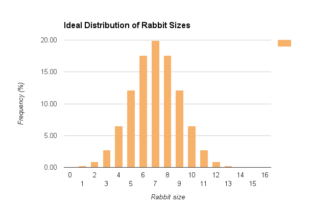
The graph above tell us that ideally there should be a nearly 20% chance for a rabbit to be exactly 7 units in size, ~17% of a rabbit being size 6 (and same chances of being 8) ~12% chances for size 5 (and same for 9), and so on. We could play with the standard deviation to change how closely we want most rabbits to be to the “average” size, but I’m quite happy with the distribution above.
Please also note that between 5 and 9 we have around 78% of the samples, which is more than the 68% we said before was normally contained in the interval between (mean – sd) and (mean + sd). This is because this is a discrete (i.e; non-continuous) distribution, and values from the vicinity of 5 and 9 are aggregated into their probabilities.
Ok, so… how do we get that in a game? In this case I’d like to discuss how to achieve that in small groups first, because ironically enough, that’s actually simpler taking into account what we’ve seen so far.
Almost-Perfect Gaussian distribution for small sets
I really like how exciting the title sounds, and how disappointingly simple the solution to this problem is.
Remember the method I introduced by the end of my previous post to get uniform distributions on small sets? Well, it turns out it can be used to get numbers that follow any distribution you want, with no modification except for the starting pool of numbers.
In the example I gave, where we had a pool of 20 numbers to draw from, I populated the set with this code:
for (i=0;i<RND_POOL_SIZE;i++) random_set[i] = (i % 10) + 1;
As the size of the pool was 20, our set ended up looking internally like this:
{1, 2, 3, 4, 5, 6, 7, 8, 9, 10, 1, 2, 3, 4, 5, 6, 7, 8, 9, 10}
Which is a perfectly uniform set, where every number from 1 to 10 appears twice.
I can compute the expected frequencies for the same range of values (from 1 to 10) following a normal distribution with -let’s say- a mean of 5 and a standard deviation of 1, and approximate how many times they should appear in a set of 20 numbers, and then manually initialize the array. In this example an array that follows more or less this distribution would be:
{1, 2, 2, 3, 3, 4, 4, 4, 5, 5, 5, 5, 6, 6, 6, 7, 7, 8, 8, 9}
You can input those values by hand in the code or create a function that fills the initial pool for you, computing the frequencies for each value following a normal distribution (using the norm() function previously defined), and then pushing a proper amount of that value into the array. For example, given the parameters above (mean: 5, sd: 1) “5” should have a 20% probably of being drawn, which for a set of 20 numbers means it should be added 4 times to the pool.
As values had to be severely rounded up or down due to the small sample size, this is more of an approximation to a Gaussian curve, and in the long run will accumulate big differences against a real normal distribution, but for small sets this gets the job done, and you can even add numbers following any wild random distribution you want to the array, and the method outlined will still work flawlessly.
Large-scale Normal Distribution
Of course you can’t get away with the previous method when you need to draw thousand of samples following a normal distribution. There’s actually a few algorithms to do that, but I will show you a favorite of mine, which I consider incredibly clever and practical.
The Box-Muller Transform
The method I’m talking about is called the Box-Muller transform and the only thing it requires is a uniform deviate (this is, a random variable that follows a uniform distribution, like all the algorithms we saw in Part 1) and gives us a series of numbers that conform to a standard normal distribution as a result. This algorithm requires the random variable (your PRNG of choice) to be in the [0.0, 1.0] range, so you will need a function like this:
double uniform_rnd(){
  return rand2() / (RAND2_MAX + 1.0);
}
To be fair it’s way easier to deal with random methods if their output is in the [0.0, 1.0] range, so this is a handy function to have in your codebase.
Due to the narrow interval required I recommend you to use something other than the standard rand() here. We want as much precision as possible, and a compiler with a poorly-coded rand() may end up botching the distribution. Replace rand2() and RAND2_MAX in the code above with the implementation of a regular PRNG of your liking.
From this uniform distribution the Box-Muller algorithm will generates 2 numbers each call, so you can either save the second one for later (as a sort of buffered value) or you can use this feature to generate a random 2-dimensional point in space in a single call (useful for example in image processing algorithms).
Another interesting thing of this method, is that it can be implemented as a mapping function to a polar space in a way that does not require trigonometric functions, which helps with its portability.
The Polar version of the Box-Muller transform in C looks like this (code adapted from “Numerical Recipes in C”):
int    rnd_n_avail = 0;
double rnd_n;
double std_normal_rnd(){
  double fac, rsq, v1, v2;
  if (rnd_n_avail == 0) {	/* No number available in buffer */
    do{
      v1 = 2.0*uniform_rnd()-1.0; /* Component in the [-1,1] range */
      v2 = 2.0*uniform_rnd()-1.0; /* Component in the [-1,1] range */
      rsq = v1*v1+v2*v2;
    }while(rsq >= 1.0 || rsq == 0.0);
    fac = sqrt((-2.0*log(rsq))/rsq);

    /* Save the first number for the next call */
    rnd_n = v1*fac;
    rnd_n_avail = 1;
    /* Return the second one */
    return v2*fac;
  }else{
    /* Return the computed one */
    rnd_n_avail = 0;
    return rnd_n;
  }
}
The function above returns numbers following a standard normal distribution, so we will need to use our previously gained knowledge to convert this to any range we want, transforming the output using the procedure I introduced earlier that takes the 2 parameters we now know and love:
double normal_rnd(double mean, double sd){
  return std_normal_rnd()*sd + mean;
}
Using the code above I will now generate a population of 10.000 samples following the distribution I defined earlier for our group of rabbits (expected size: 7, standard deviation: 2), counting how many times each size was generated and later plotting the results:
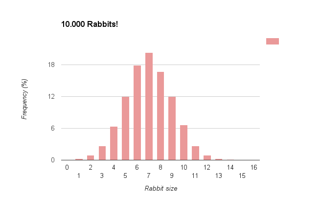
Of course the more numbers we draw from the generator, the more the graph will match the Gaussian curve we computed before, but even with a set of moderate size it already shows that we are successfully generating a list of numbers that follow the distribution we were after.
There are many other distributions, of course, and there are algorithms for all of them, but I’d say we just covered the most important and common one, and hopefully this will be useful for you in your games or future projects.